Before
After
I have developed several computer simulations for an undergraduate course I teach at Indiana University called "Complex Adaptive Systems." The course deals with systems that evolve and adapt over time. Psychology, computer science, economics, biology, and neuroscience depend upon a deeper understanding of the mechanisms that govern adaptive systems. A common feature of these systems is that organized behavior emerges from the interactions of many simple parts. Ants organize to build colonies, neurons organize to produce adaptive human behavior, and businesses organize to create economies. To address the essential question of "What are the properties of complex adaptive systems?," case studies of several systems are explored: chaotic growth in animal populations, human learning, cooperation and competition within social groups, and the evolution of artificial life. The central thesis is that widely different systems (businesses, ant colonies, brains) share fundamental commonalities.
These topics will be explored by extensive hands-on use of interactive
computer simulations. The basic problem with teaching complex systems
is that they are .... complex. Appreciating how structured,
organized behavior can emerge from the interactions of many units is almost
impossible unless one can create a working model of these interactions.
Similarly, it is hard for students to understand how simple mathematical
equations can explain how the brain is organized, how populations grow
and shrink, and fires spread (to take three arbitrary examples), unless
they can experiment with these equations, and if they can see the results
of these experiments in a graphic, intuitive manner. By experimenting
with computer simulations, students can bridge the gap between mathematical
formulae and large-scale behavior. The philosophical motivation of
pedagogy for these simulations is:
All of the programs on this page are written for Macintosh computers.
They should work on any powermac, but several of them are computationally
demanding, and will run slowly on anything more feeble than an Imac or
G3. The optimal screen size is 1024 X 768.
Two students working with me have ported over some of these Macintosh simulations to be Java applets, with the intention of creating platform-independent simulations. Stay tuned as more of the simulations are ported over to Java. For now, check out the simulations by these students:
Press here to download Ball Dropper
Press here to download Path Finder
Press here to download Resource Cover
Press here to download Pattern Learner
Press here to download Predators and Prey
Press here to download Hebbian Learning
Press here to download Pine Cone
Press here to download Input/Output Learning
Press here to download Traveling Salesman
Press here to download Apparent Motion
Press here to download The Chaos Game
Press here to download Learning Facilitating Evolution
References and Further Reading for Simulations
What follows is a brief description of the currently available complex
system simulations
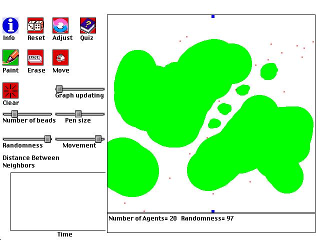
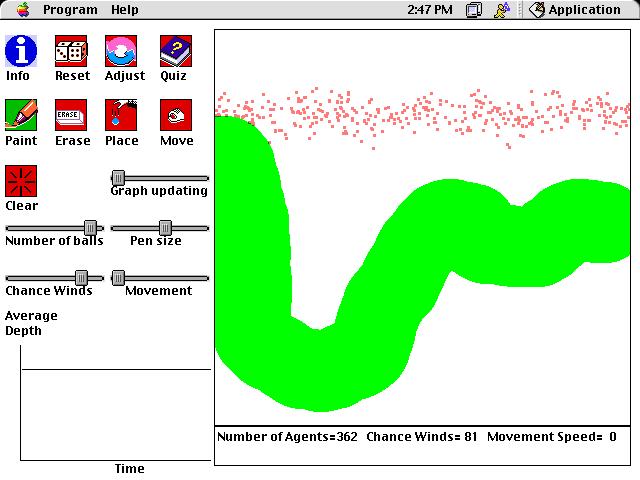
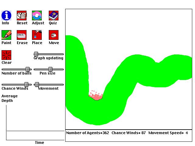
Ball dropper
This is a computer simulation of balls falling
on a windy day. It was designed to teach students about local and
global minima, and the effectiveness of a "simulated annealing" schedule
for finding global minima. In this simulation, simulated annealing
involves gradually reducing the amount of randomness in the balls' motions.
Each ball follows a few simple rules:
1. The balls will generally fall downwards.
2. The balls will also be influenced by a random factor.
3. The balls will not pass through anything painted green.
As a goal, imagine that you are trying to have all of the balls
drop as low as possible. How can this be done? Even though
the wind is random, you can use it to help you.
Experiment with dropping balls on different landscapes. Do the balls find the lowest possible spot in each landscape? If they don't, why not?
Experiment with different ways of adjusting the amount of randomness and amount of movement of the balls. What technique does the best job of putting the balls at the lowest spot?
How can you avoid having your balls settle in shallow valleys when deeper valleys exist?
Before
After
Path Finder
This is a computer simulation of balls influencing each other, and
as a group, finding pathways around obstacles. It also demonstrates
notions related to local and global minima, and simulated annealing.
In fact, the reason for including both "Ball Dropper" and "Path Finder"
is to demonstrate how the same abstract principle may apply in different
domains, and to train students in skills related to extracting underlying
abstract similarities. The balls follow the following simple rules:
1. Each ball is assigned two neighbors, making a set of balls arranged from first to last. One of the fixed blue points is the neighbor of the first ball. The other blue point is the neighbor of the last ball.
2. Each ball will move toward of its two neighbors, and will also move with a bit of randomness.
3. If the location that a ball would move to is painted green, then it does not move.
With these simple rules, and the right setting of parameters,
it is possible to have the balls find a pathway that connects the two blue
endpoints and avoids the green obstacles.
Experiment with different ways of adjusting the amount of randomness and amount of movement of the balls. What technique does the best job of usually finding good pathways?
Here are some other questions to ponder as you play with this simulation:
What is the best number of balls for a maze? Why? What kinds of mazes can and cannot usually be solved? If the balls have trouble finding a pathway, what can you do to help them?
Before

Press here to download Path Finder
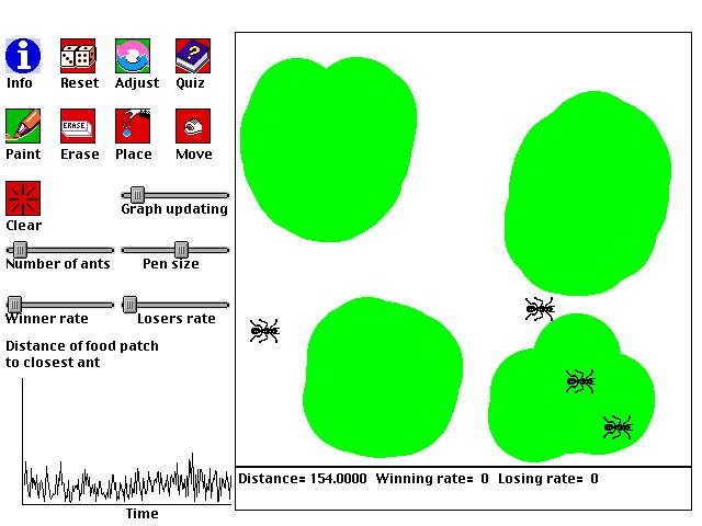
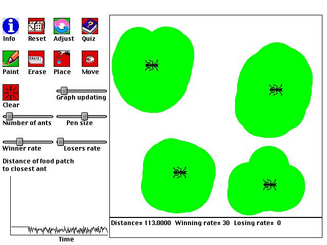
Resource Cover
This is a computer simulation of ants covering food that is placed down, or more generally, any set of agents trying to optimally cover a set of resources (e.g. oil drills covering an oil field, or scientists covering a domain of inquiry). The following simple steps determine the behavior of the ants:
1. One piece of food (green pixel) is randomly selected from all the food present.With these simple rules, and the right setting of parameters, the ants will often arrange themselves so that they optimally cover the available food. That is, the ants move so that the distance between every piece of food and its closest ant is as small as possible. The food is well covered. For example, if there are two ants and two food sources, generally speaking each ant will cover one of the food sources.
2. The ant that is closest to the selected food moves toward the food with one speed.
3. All of the other ants move toward the food with another speed.
Experiment with different ways of adjusting how quickly the ants move. What technique does the best job of usually helping the ants cover the food optimally?
Here are some other questions to ponder as you play with this simulation:
Why don't you want to move the ants as quickly as they can go? If you have 5 ants, and one region of food is 4 times bigger than another, how do the ants distribute themselves? If you make two food piles and place two ants in one pile, what can you do to make the ants find different piles, and why does this work?
After
Press
here to download Resource Cover
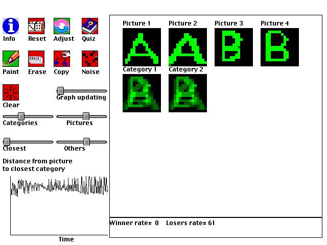
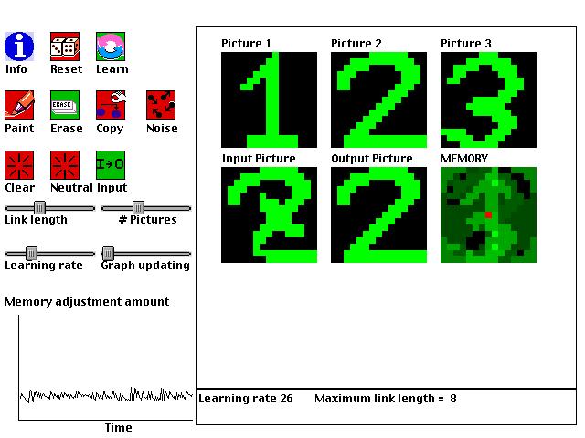
Pattern Learner
This is an example of a type of artificial intelligence called a "neural network." It shows how a computer can learn to categorize pictures even without a person telling it what pictures belong together. For example, if a person draws pictures of "A"s and "B"s, the computer may create two categories, one for each letter. As with the first pair of simulations, this simulation is abstractly related to the previous "Resource Cover" simulation. Both simulations involve finding ways to optimally cover presented information by creating agents that are specialized for subsets of the information.
As a person paints different pictures, the computer will create categories, using the following simple steps:
1. The person tells the computer how many pictures and categories to allow.The computer automatically forms categories that include pictures that look most alike, and the categories emphasize the parts that are shared by all of the pictures belonging to the category.
2. A picture is randomly selected.
3. The category that is closest to the picture adapts itself to the picture by a certain amount.
4. All of the other categories adapt themselves to the picture by a different amount.
As you use this neural network, try to figure out how the computer is able to automatically form categories of pictures simply by using the steps just described. Try situations where the number of categories is the same as the number of pictures, and also situations where there are fewer categories than pictures.
Here are some other questions to ponder as you play with this simulation:
Why aren't good categories found when all of the categories adapt equally quickly to selected pictures? If there are two categories and two pictures, what can you do to make the two categories each become specialized for a different picture, and why does this work? Once each category is specialized for one picture, make a change to one of the pictures. Why does only one category (the correct one) change?
After

Press here to download Pattern Learner
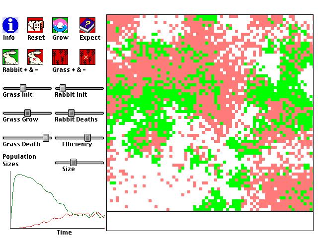
Predators and Prey
This is a computer simulation of the changes in populations of predatory and preys. An historical example is the cyclic variation of lynx and rabbit populations. However, we will consider populations of rabbits and grass because their interactions are better modeled by the equations used here. Often it is observed that as the amount of grass grows in a regions, the population of rabbits will increase with their food source. However, as the rabbit population increases, the grass population will decrease from over-harvesting. Then, the population of rabbits will decrease because of the dwindling food supply of grass. With fewer predators, the grass population increases again, perpetuating the cyclic population variation.
Around 1926, Lotka and Voltera independently
came up with following two equations two describe the dynamics of predator-prey
populations:
dG/dt = a*G - b*G*R
dR/dt = d*b*G*R - c*R
where:
a=growth rate of grass without predation
b= rate of consumption of grass by rabbits
per encounter
c = natural death rate of rabbits
d = efficiency of turning grass into new rabbits
dG/dt and dR/dt are the rates of change of the grass and rabbit populations from one instant to the next. As such, the populations of rabbits and grass only depends on the immediately preceding population sizes.
One way of modeling populations is simply to
apply the Lotka-Voltera equations given a set of four parameters.
The computer will show this simulation when asked to show the "expected
populations" according to this model. A dynamical, graphical simulation
of these equations is also provided. This simulation proceeds by
the following rules:
1. Initial populations of rabbits and grass are set by parameters. Organisms are randomly positioned in a field with a size set by the user.
2. For each patch of grass, if a random number between 1 and 100 is less than the "grass grow rate" (parameter "a" of the Lotka-Volera system) then a new piece of grass is created near the grass.
3. For each rabbit, if a random number between 1 and 100 is less than the "rabbit death rate" (parameter "c") then the rabbit will die.
4. If a rabbit is on top of a patch of grass, and if a random number between 1 and 100 is less than "rate of consumption" (parameter "b"), then the grass will die, and the rabbit will give birth to another rabbit if another number between 1 and 100 is less than the "efficiency rate" (parameter "d"). The new rabbit will be placed next to the old rabbit.
5. Each rabbit and grass will randomly move to an adjacent square.
There is a limit of 20,000 rabbits or grass,
and this limits how many pieces of grass can co-exist on the same patch
(capacity = 20,000/number of patches).
You will notice that, for any combination of parameters, the populations predicted by the Lotka-Voltera equations are not the same as the populations predicted by the graphical population model just described. One of the main reasons for this is that the Lotka-Voltera equations have no notion of space. All predators and preys are imagined to be on the same patch. One consequence of this is that predators are much more likely to die out in the graphical/spatial model, because they will be less likely to be standing on a grass patch at any given time. It may be that the graphical model is a more realistic simulation of populations. It can be shown that the Lotka-Voltera equations always (see below for one exception) predict cyclic, rather than relatively stable, populations. Population cycles are found in nature, but not always.
The spatial model of populations predicts many more relatively stable populations. Why?
Other things to think about:
For pure fun, let a crop of grass grow
without any rabbits, and set "grass grow rate" to 1. Now, try to
eliminate all grass with the "erase grass" tool. Can you do it?
What if "grass grow rate" = 2? Why the big change?
Press
here to download Predators and Prey
Hebbian Learning
This is an example of a type of artificial intelligence called a "neural network." It shows how a computer can be trained with some pictures, and can then later recognize distorted versions of the pictures. A single memory is used to store information from all of the presented pictures. The memory is "distributed" in that all parts of the memory are used for representing all of the pictures, rather than having each picture in its own memory. The memory of the network consists only of connections between each pixel of a 15 X 15 grid to each other pixel (thus, it is made up of 50,625 numbers). Every pixel in a picture takes on a value between -1 and 1. Each connection in memory describes the relation between two pixels. If the pixels tend to be in the same state, then the connection will be positive; If they are in different states, the connection will be negative. Memories are learned using a modification of the Hebbian learning rule (named after Donald Hebb, a Canadian neurophysiologist). According to this modified rule:
The change in the link between pixels A and B is proportional to (1) the product of their states, (2) a learning rate, and (3) the difference between the current link and the minimum or maximum value a link can take.Term (1) adjusts the link in the correct way, increasing the link for positively correlated pixels, and decreasing it for negatively correlated pixels. Term (3) makes sure that the links don't grow without bounds.
This learning rule shows the following useful behaviors:
All of these properties can be traced to
the simple rule for creating memories, and the simple rule for changing
pictures by the learned memories.
While experimenting with the simulation, try the following:
Create a picture, and then see how distorted versions the picture are "cleaned up." Create two pictures, and see how the memory can retain traces of both at the same time. If you feed something that looks like one of the pictures, it will become more like whichever stored picture it is more similar to. Trying limiting the distance that links can reach, and feeding in a small part of picture (try feeding in the picture with both black and neutral green backgrounds). How is the complete picture reproduced?
Before
After
Press
here to download Hebbian Learning
Pine Cone
This is a computer simulation of how some elegant
mathematical relationships commonly found in plants emerge. Many
of the relationships are based on the Fibonacci sequence:
1, 1, 2, 3, 5, 8, 13, 21, 34, 55, 89, 144,
...
where each number is obtained by adding together
the two previous numbers.
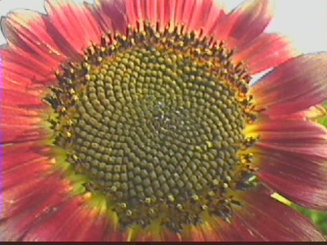
Seeds are often arranged in spirals on flower heads. Often times there are both noticeable counterclockwise and clockwise spirals. The number of spirals going in one direction is usually one of the numbers from the Fibonacci sequence. The numbers of clockwise and counterclockwise spirals are usually SUCCESSIVE NUMBERS in the Fibonacci sequence. For example, a sunflower may have 21 clockwise spirals and 34 counter clockwise spirals. Below, you'll see an actual photograph of a sunflower from http://www.sunflowers.com/. With a little effort, you can probably see patches where there are counterclockwise and clockwise spirals, and you may even be able to count the number of each type of spiral (I count 34 clockwise spirals).
Another place where the Fibonacci sequence emerges is if we examine each of the spirals more closely. We can number each plant element (seed head, petals, needle, etc.) by when it was formed. For example, the first "petal" on a pine cone would be 1, the second is 2, etc. All of the petals that lie on a spiral are a constant number of petals apart. These constants are numbers from the Fibonacci sequence. Furthermore, the constants associated with the counterclockwise and clockwise spirals will be SUCCESSIVE numbers from the Fibonacci sequence.
A final, related mathematical fact is that successive elements of a plant are often separated by 137.5 degrees. This is an interesting number, because it is the equivalent of the golden section for a circle. The Golden Section, Phi, a mathematical phenomenon known and used architecturally by the ancient Greeks, is the only number that when squared, is simply equal to itself + 1. That is, Phi*Phi = Phi+1. Plants very often send off leaves, seeds, stems, etc. at angles based on the Golden Section. What is the relation to the Fibonacci sequence? The ratio of successive numbers of the Fibonacci sequence becomes a better and better approximation to Phi as the sequence continues. For example, 13/8 = 1.625, 21/13 = 1.615..., and 34/21 = 1.619..., while Phi=1.618033989...
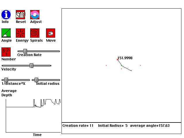
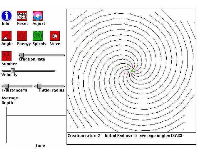
The current simulation is based on Doady and Couder's (1992) work on modeling plant growth. The basic idea is that the next plant element to be formed will be formed where there is the most space. Plant elements will be formed somewhere on the radius around the center of the plant. They will move away from the center with a certain velocity. They will be created at a certain rate. Those three parameters (radius, velocity, creation rate) will determine how the entire plant's growth appears.
The following simulation creates plant forms by the following simple steps:
1. Place the next plant part at point P on Radius R around the center where energy is at a minimum.
That is, energy will be the sum of an inverse function of the distances between the point P and the other, already existing plant parts A. Thus, a point P will be selected for the next plant part if it is, on average, the farthest point on the radius from existing parts.2. For plant parts that have already been formed, move them away from the center with a parametrically determined velocity, in the same direction as they were originally placed.
By executing these simple rules with different parameters, many
common plant types can be created, from the simple alternating leaf arrangement
of corn to the complex seed head spirals of daisies and sunflowers.
Try experimenting with different parameters, and see if you can get parts
separated by 137.5 degrees, or spirals related to Fibonacci numbers.
Before
After
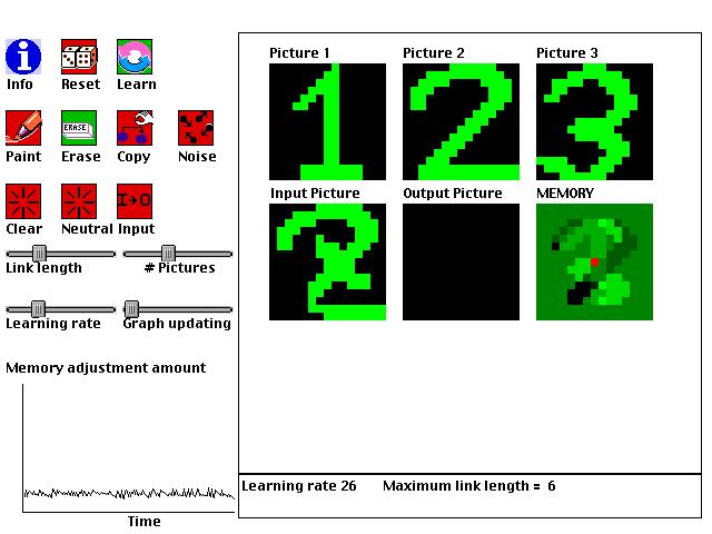
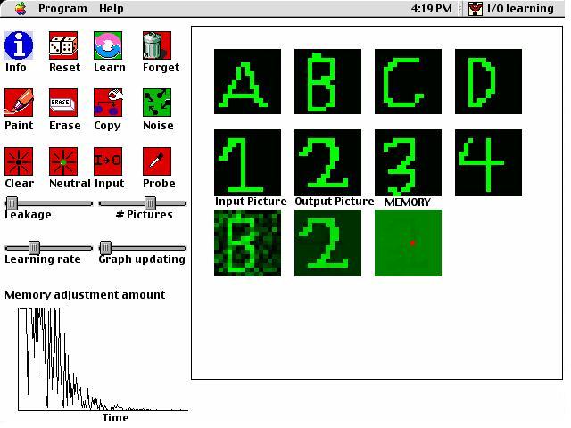
Input/Output Learning
This is an example of a type of artificial intelligence called a "neural network." It shows how a computer can learn to associate several pairs of input and output pictures to each other. A single memory is used to store information from all of the presented pictures. The memory is "distributed" in that all parts of the memory are used for representing all of the input/output pairs. The memory of the network consists only of connections between each pixel of a 15 X 15 grid to each other pixel (thus, it is made up of 50,625 numbers). Every pixel in a picture takes on a value between -1 and 1. Each connection in memory describes the relation between two pixels. If the pixels tend to be in the same state, then the connection will be positive; If they are in different states, the connection will be negative. Memories are learned using the Delta Rule (McClelland & Rumelhart, 1986). This net input is compared to the desired output - the actual value of the pixel in the output picture. The bigger the difference between the desired output and the net input to the pixel, the greater the change in connections will be. According to this rule, if the net input to a pixel is greater than the pixel's actual state of activation, then the change in the weight from i to j will be negative. This means that if Pixel i is active, then its connection to j will decrease, which is desireable because it means that the next time i is active, it will not cause j to become so active. Conversely, if the net input to Pixel j is too small compared to the actual state of j, then the change of weight will be positive, making an active unit i more potent in activating j. After weights between units have been learned, they affect the later behavior of the neural network. When given a certain set of input activities, the behavior of the network will be equal to the net input to each output unit.
The delta rule of neural network learning has a number of useful properties:
Before
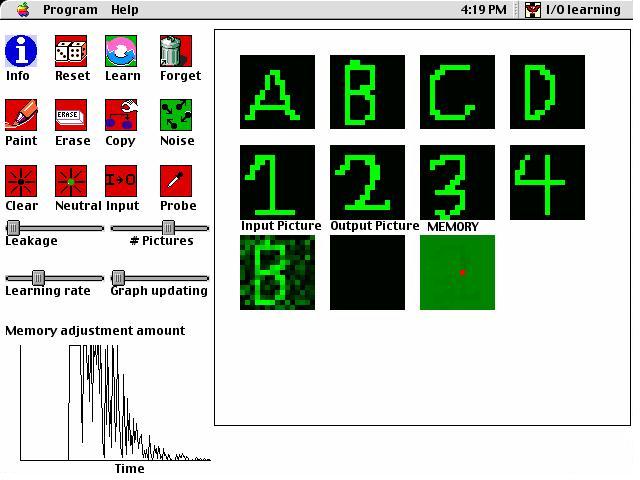
After
Press
here to download Input/Output Learning
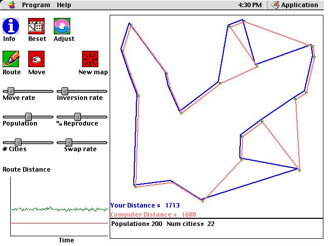
Traveling Salesman
This computer simulation solves the classic "Traveling Salesman" problem. The goal of this problem is to find the shortest possible route between N cities, visiting each city once and returning to the starting city. Finding the route which is definitely the shortest possible route is known to be an NP-Complete problem, meaning that as the number of cities increases LINEARLY, any computer algorithm requires an EXPONENTIALLY increasing number of steps. NP-complete problems are thus considered to be intractable, but that does not mean that reasonable solutions for them cannot usually be found. There is no guarantee that these "reasonable" solutions will be the very best possible, but typically they will be very close to the optimal solution if reasonable parameters are chosen. In this simulation, there is a population of solutions, each of which offers a particular route through a set of cities. The entire system can develop a good solution for a given map of cities by selectively "breeding" solutions. Thus, the set of solutions evolve over time. Each new generation will be based on the previous generation, but with a bit of variation thrown in. The computer will show the best (most "fit" in evolutionary terms) solution among those available in a particular generation. Unlike typical computer searches for a good solution, here an entire POPULATION searches for a solution, meaning that the system tends not to get stuck in dead-ends as easily as systems with only a single agent that is searching.
Each solution within a population consists
of a simple representation of a route among cities. Namely, it is
an ordered set of N numbers where each number identifies a city.
If an agent's set is: 5 7 2 3 1 6 4
then the route would go from City 5 to City
7, and then to Cities 2, 3, 1, 6, 4, in order, and then would finally return
to City 5. By changing ("mutating" to use the evolutionary term)
its solutions, a system can explore different solutions to a map.
Here are the particular types of mutation allowed in this program:
While exploring this simulation, here are some questions to consider:
Before
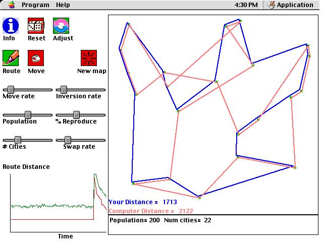
After
Press
here to download Traveling Salesman
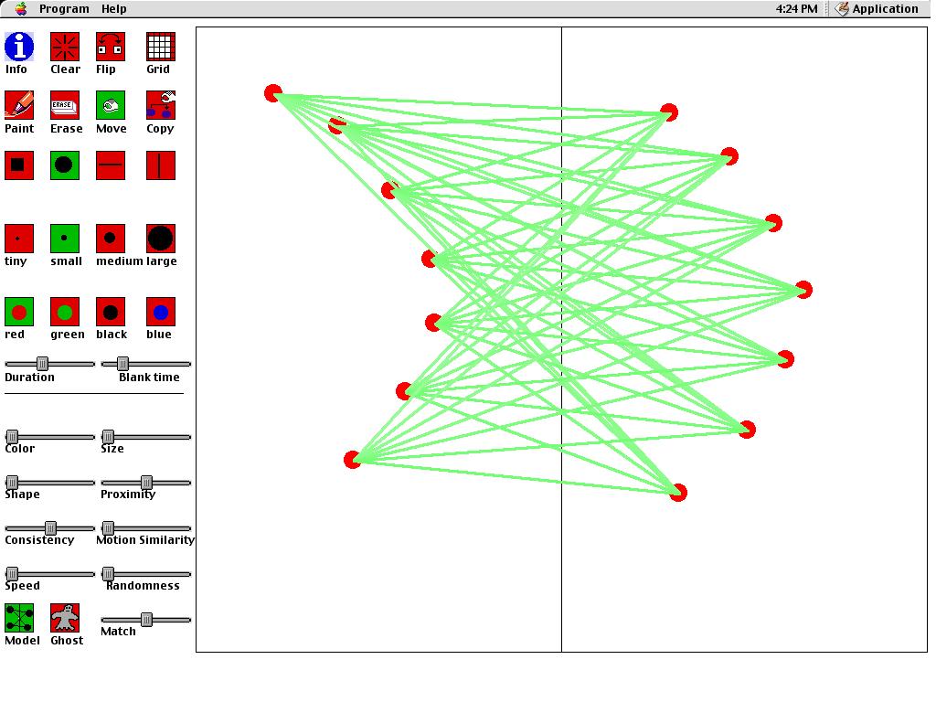
When static pictures are rapidly alternated, people often spontaneously perceive illusory motion. By studying apparent motion phenomena, we can learn about how people subjectively structure the external world , the assumptions that people make about stimuli when perceiving, top-down effects in vision, and the specific mechanisms that people use to see motion. Apparent motion is also indispensible to the motion picture industry because movies are nothing more than a series of still frames that are rapidly displayed.
This program does two things. First,
it allows you to create and display apparent motion phenomena. You
can design an apparent motion display, and then present it to yourself
and determine the motion that you spontaneously see. Second, it provides
a computational model of how people see apparent motion. Typically,
you will use this program by presenting the same apparent motion display
to yourself and to the computational model, and observing whether the computer
"sees" the same kind of motion that you do.
When people see motion between two successively
presented frames, their minds unconsciousnly determine which parts
from the first frame correspond to which parts from the second frame.
When people see two parts as corresponding to each other, this means that
they interpret the two parts as coming from the same object. If the
two parts are separated from each other, then people will see a single
object moving over time.
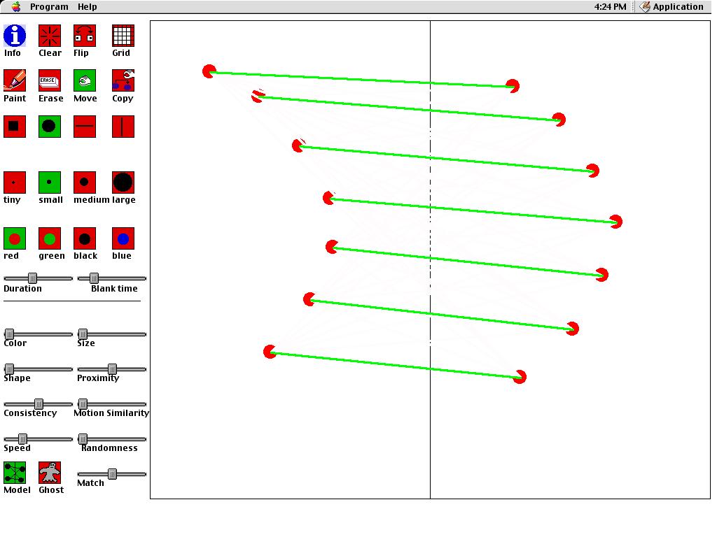
Determining what parts correspond to each other
tells us what parts come from the same object at different times.
However, this task is intrinsically ambiguous. One part in one frame
could correspond to many different parts in the other frame. Simple
experiments will show that people sometimes see two parts as showing the
same object moving over time even if the parts do not have the same color,
size, location, or even shape! Your mind spontaneously figures out
what parts correspond to each other, but underlying is seemingly effortless
feat are sophisticated computations. Your mind uses several constraints
in order to try to determine what parts correspond to each other.
Before
After
Press
here to download Apparent Motion
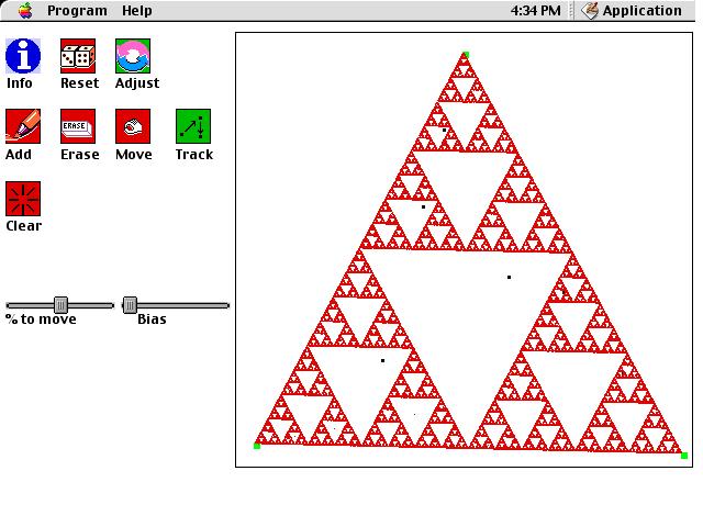
This is a computer simulation of "The Chaos Game." This simulation obeys the following rules:
The main puzzle to try to solve with this simulation is: Why
does the random procedure for moving points from time to time produce Sierpinski's
gasket? With a bit of exploration and thought, you can probably figure
out the reason. To help you, we have provided a feature that allows
you to plot a point, and click on endpoints to simulate how the point would
move if the endpoint was chosen. Once you understand the behavior
of the system, a more challenging question is to try to determine the AREA
of the plotted region as the number of iterations goes to infinity.
Press
here to download The Chaos Game
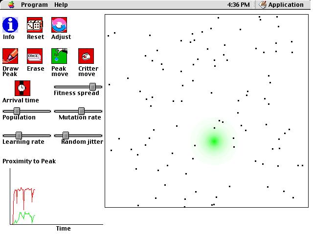
This is a computer simulation of the "Baldwin Effect." By this
effect, evolution proceeds at a faster rate for species if they are made
up of organisms that can learn. This statement of the Baldwin effect
may seem suspiciously similar to the Lamarckian theory of acquired characteristics,
by which adaptations within an organism's lifetime are passed down to its
children. For example, Lamarck argued that giraffes who continually
reach for high leafs on trees stretch their necks over time. The
neck's new length will be passed down as a physical characteristic to the
giraffe's children. It is now known that characteristics are not
acquired in this way. Physical changes to an organism that occur
in its lifetime do not affect its genetic code, and this is what is passed
down to the next generation. However, the Baldwin effect HAS been
observed. What an organisms learns during its lifetime does influence
the course of evolution for the species. This goal of this simulation
is to show how this is possible.
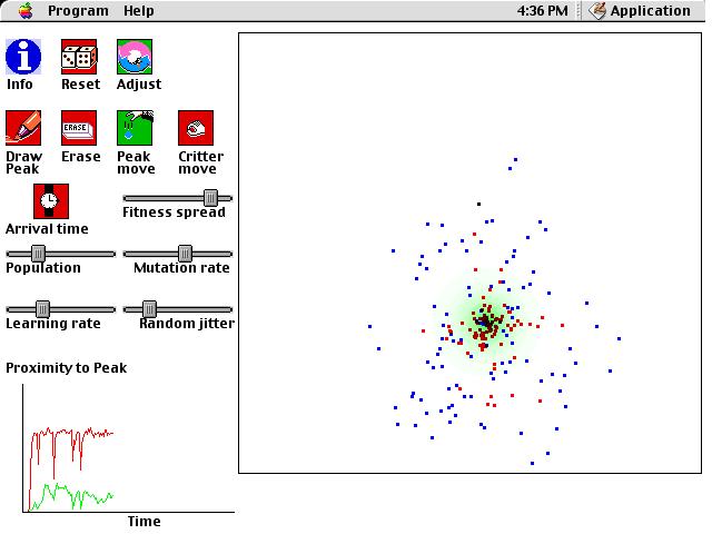
Continuing to simplify matters, we will also represent organisms
by points in space. Their genetic code will define their starting
locations, and in their lifetime, they may move their location if they
are endowed with an ability to learn. If they can learn, they will
generally move toward the closest fitness peak to them. For example,
an organism may start off life unable to scratch its head to clear off
fleas, but it may gradually get better and better at doing this.
As you explore the simulation, remember that the initial location
for an organism before it starts learning can be considered to be its genetic
code. These locations, shown in blue, may change over the course
of generations. This would be evidence for evolution of the entire species.
Thus, there are two types of change to observe. There is learning
within a single organism's lifetime, indicated by moving red dots.
There is also evolution of the genetic code of the entire population, indicated
by distributions of blue dots.
Under what circumstances does learning facilitate evolutionary change? One factor that matters considerably is whether the fitness peak is more like a vertical spike or a gradual hill. In one of these situations, learning can allow genetic improvement to occur much more quickly than it would without learning. Which situation, and why?
There is also a situation where learning can initially cause genetic improvement, but then can later actually interfere with further genetic improvement. Why does this occur, and what can be done to prevent this interference?
How does the mutation rate influence the Baldwin effect? What are the costs and benefits of a high mutation rate?
Once a population has evolved well to a fitness peak, try moving the fitness peak far away. What factors allow the population to quickly adapt to the new peak, and why do they work this way?
Compare changing the learning rate to changing the random jitter in organisms. Do BOTH types of variation produce a Baldwin Effect? Why or why not?
Assuming that mutation rates can be modified in evolutionary time, what does the simulation predict about the relative mutation rates for populations that are close to a fitness peak versus far away?
After
Press here to download Baldwin
hits
since 9/22/01
![]()
Date last modified: 9/27/2001